Matrix Multiplication Feels Bad
In our last post we talked about the implications of both sequential and parallel naive Matrix-Matrix multiplication (MMM). Sadly we found that this classic triple for-loop approach suffers from poor locality.
 OMG, who would have known? Our algorithms actually sometimes need to be cache-aware.
This time around we will look at the tall cache assumption along with loop-tiling applied to parallel and sequential MMM. As you would expect there are also some pretty benchmarks involved.
Cache-Awareness, So Confuse
In easy terms, most of the transfers between cache and disk simply involve blocks of data. Whereby the disk is partitioned into blocks of B elements each, and accessing one element on disk copies its entire block to cache. When assuming a tall cache, the cache can store up to M/B blocks, for a total size of M elements, M ≥ B².
Meaning when the cache is already full and a block is grabbed from disk, then another block will be evicted from cache. Before exploring something more cache-aware let us demonstrate this occurring in our naive (and cache-oblivious) solution. Assuming square matrices which do not fit into a tall cache then
n = rowAmountOfA = colAmountOfA = rowAmountOfB
n > M/B
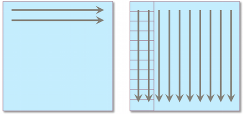
Bellow we see the row-major layout of matrices A and B. We depict the red rectangles in matrix B as our blocks of cache. For all rows of matrix A we traverse over each column of B. Upon traversing B the accessing of each element is cached. Given that n = colAmountOfA and n > M/B then before the traversal of a column B completes the first, and possibly several subsequent, cached blocks of B will be evicted. So upon the next and remaining traversals of B we incur cache-misses on each block
From this we can be quite clever and infer that a naive algorithm with n > M/B results gets the following work done
Q(n) = Θ(n3)
Which implies that a naive algorithm with n ≤ M/B will get the following work done since the second matrix can now exploit spatial locality
Q(n) = Θ(n3)/B
Loop-Tiling, Feels Good
Lets take a look at a standard tiling solution to resolve our cache capacity misses.

Pro tip: loop-tiling is a type of loop transformation on which many cache blocking algorithms are built.
It involves a combination of strip-mining and interchange in multiply-nested loops, in turn strip-mines several nested loops and performs interchanges to bring the strip-loops inward.
This following tiling solution ensures greater spatial locality for accesses across matrix B. Simple but effective, our implementation partitions the matrices’ iteration space though such strip mining and loop interchange
s = (int) Math.ceil(rowAmount1 ∗ 1.0 / 4);
s2 = (int) Math.ceil(colAmount1 ∗ 1.0 / 4);
s3 = (int) Math.ceil(rowAmount2 ∗ 1.0 / 4);
for (i = 0; i < rowAmount1 / s; i+=s){
  for (j = 0; j < colAmount1 / s2; j+=s2){
    for (k = 0; k < rowAmount2 /s3; k+=s3){
      for (i2 = i; i2 < (i+s) && i2 < rowAmount1; i2++){
        for (j2 = j; j2 < (j+s2) && j2 < colAmount1; j2++){
          for (k2 = k; k2 < (k+s3) && k2 < rowAmount2; k2++){
            C[i2][j2] += (A[i2][k2] ∗ B[k2][j2]);
                          ....
Although not implemented recursively, tiling shares some similarities to the divide-and-conquer approach in that it aims to refine the problem size through partitioning the problems (matrices) into subproblems (submatrices). The design of the tiling solution quite naturally lends itself to parallelisation. Such is implemented as follows
s = (int) Math.ceil(rowAmount1 ∗ 1.0 / 4);
s2 = (int) Math.ceil(colAmount1 ∗ 1.0 / 4);
s3 = (int) Math.ceil(rowAmount2 ∗ 1.0 / 4);
executor = Executors.newFixedThreadPool(10);
for(interval = 10, end = rowAmount1,
size = (int) Math.ceil(rowAmount1 ∗ 1.0 / 10);
interval > 0 && end > 0; interval−−, end −= size){
to = end;
from = Math.max(0, end − size);
Runnable runnable = new Runnable(){
@Override
public void run() {
for (i = from; i < to / s; i+=s) {
for (j = 0; j < colAmount1 / s2; j+=s2){
for (k = 0; k < rowAmount2 /s3; k+=s3){
for (i2 = i; i2 < (i+s) && i2 < rowAmount1; i2++){
for (j2 = j; j2 < (j+s2) && j2 < colAmount1; j2++){
for (k2 = k; k2 < (k+s3) && k2 < rowAmount2; k2++){
C[i2][j2] += (A[i2][k2] ∗ B[k2][j2]);
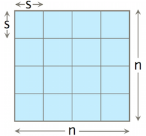
...It is important to note the s, s2 and s3 parameters to our tiling algorithm. Above we see that they are derived respectively from a matrix dimension divided by 4. They are then later used to determine the dimensions (size s2xs3) of the submatrix-submatrix multiply tasks to be ran. In the case of a square MMM the submatrices’ dimensions would be sxs.
We divide up these multiply tasks through from/to bounds - requiring no synchronisation as no mutable data is shared across threads.
Determining values for s, s2 and s3 is not straight-forward, they ultimately determine the tiling size which in turn demands an accurate estimate of the cache size on your target machine. Assuming square matrices which do not fit into a tall cache then
n = rowAmountOfA = colAmountOfA = rowAmountOfB
n > M/B
Once we determine s ≤ M/B we can easily decompose submatrices (tiles) from matrix B that respect the target cache size
As you would expect the tiling optimisation still results in Θ(n3) computations. With an optimal s value, Θ(M½), we see an improvement in the amount of work done to that of our naive approach. The tall-cache assumption implies that each submatrix and its data will fit in cache, meaning only cold caches misses should occur per submatrix (Θ(s2/B)).
Θ(n) = Θ((n/s)3(s3)) = Θ(n3)
Q(n) = Θ((n/s)3(s2/B)) = Θ(n3/BM½)
From the above, as you might have guessed, we can see that s is actually a “tuning” parameter for cache-awareness. In our solution this tiling dividend is set to 4 which, from some rudimentary testing, is the optimal value on recent i5 and i7 processors (OS X 10.10).
Dem Benchmarks: What was measured?
Our benchmarking goal was to analyse the trends displayed across the executions of naive MMM and cache-aware MMM in conjunction with parallelisation. Thus the benchmarking process undertaken had the following features:
- A varying set of dimensions for A and B respectively on both algorithms were used to identify trends. The dimensions (200x200), (200x300), (1000x1000) and (1000x1200) were used.
- To maintain measurement accuracy the elements held by A and B needed to be the same for each measurement. Every element held by A is always 2, while each element in B is always 3.
- Each benchmark was conducted on two machines (4 core and 8 cores) under the same conditions (no other user processes running, machines connected to power outlets, etc.)
Dem Results
Reflecting on the mean (μ) execution-time and according standard deviation (σ) provided by our benchmark runs, the collated results are as follows
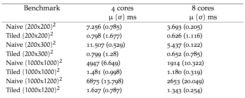
Our data poses several interesting avenues of investigation. However our main concern is exploring the benefits of cache-aware algorithms, so lets just explore the performance differences between both algorithms across runs. The bellow sidebar chart illustrates an obvious difference in our algorithms, at a glance one can see that there is large deviation between the naive and tiled time results.
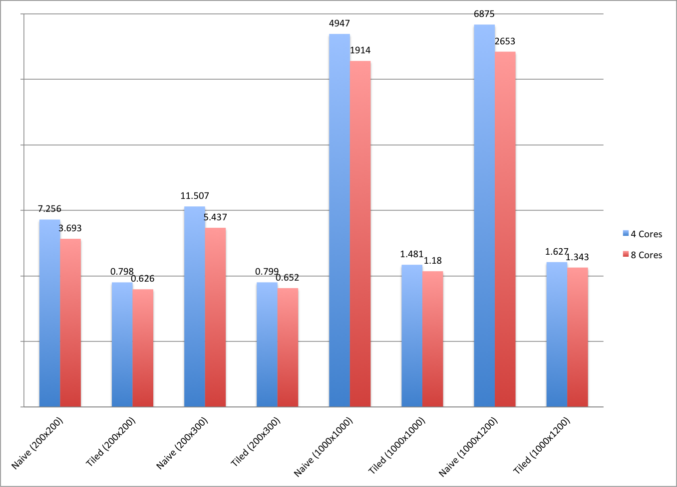
This is particularly true across the benchmarks where matrix dimensions are in their thousands. Such is unsurprising given that the naive algorithm is cache-oblivious. When viewing every sidebar related to the tiled results we can see that varying matrix dimensions do not greatly affect performance. Interestingly, we see that an increase in cores only greatly benefits the naive algorithm. It sees around a 55% improvement in execution-time with the assistance of 4 extra cores across all dimension sizes.